Bidirectional Instant Radiosity

8 Apr, 2012 #path-tracing #maths

Bidirectional Instant Radiosity is the title of a paper by B. Segovia et al which presented a new sampling strategy to find virtual point lights (VPLs) that are relevant to the camera. The algorithm given for generating VPLs is:

Generate $N/2$ "standard" VPLs by sampling light paths (i.e. vanilla instant radiosity)
Generate $N/2$ "reverse" VPLs by sampling eye paths (compute their radiance using the N/2 standard VPLs)

These $N$ VPLs are then resampled into $N^\prime$ VPLs by considering their estimated contribution to the camera. Finally the $N^\prime$ resampled VPLs are used to render an image of the scene.

In this post I'll describe how I think this approach can be generalised to generate VPLs using all the path construction techniques of a bidirectional path tracer. As usual I'm going to assume the reader is familiar with bidirectional path tracing in the Veach framework.

I should state that this is an unfinished investigation into VPL sampling. I'm going to describe the core idea and formally define the VPL "virtual sensor", but proper analysis of the results will be part of a future post (and may well indicate that this approach is not advisable).

Core Idea

Bidirectional path tracing is about generating eye and light subpaths, considering all possible ways to connect them, and combining the results using multiple importance sampling.

In order to apply bidirectional path tracing to VPL generation, it seems natural to make the start of our eye subpath a VPL. To achieve this we define a "virtual sensor" that covers every surface in the scene that is capable of being a VPL. This virtual sensor generates VPL locations as follows:

If the light subpath hits the virtual sensor (i.e. hits anywhere in the scene) this is a VPL location. (In fact these are exactly the VPL locations you would get from "standard" instant radiosity.)
When the virtual sensor is sampled (i.e. for the first eye subpath vertex), this is a VPL location.

To compute the value of each VPL, we evaluate each subpath combination using standard bidirectional path tracing with multiple importance sampling, accumulating the weighted contribution into the appropriate VPL. In this way, all possible subpath combinations are used as sampling techniques during VPL construction.

Background: Lightmapping

For the motivation of this idea, consider solving a lightmap using bidirectional path tracing. A lightmap is a sensor that sits on some surface in the scene, acting as the dual of an area light. The end result is an image that captures all of the direct and indirect lighting on the surface.

In the diagram below, we consider a bidirectional path consisting of the eye subpath $\mathbf{z}_0\mathbf{z}_1\mathbf{z}_2$ that starts from the lightmap sensor and the light subpath $\mathbf{y}_0\mathbf{y}_1\mathbf{y}_2$ that starts from a light source (i.e. the standard Veach notation).

Lightmapping Bidirectional Path

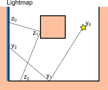
In camera renders with a physical aperture (for example with a thin lens camera model), it is unlikely that light subpaths hit the sensor. For lightmaps, the sensor is much larger, so light subpaths that hit the sensor are much more likely. Also, unlike camera renders, it is usually only the position on the surface that affects which lightmap pixel receives the sample (not the incoming angle).

As such, for a lightmap sensor, the location of a weighted sample to be accumulated into the final image is always defined by the last (in the sense of paths going from lights to sensors) vertex of the bidirectional path. Only certain vertices can be the last vertex, namely:

$\mathbf{z}_0$ : this is the first vertex of the eye subpath, which we obtained by sampling the lightmap sensor
$\mathbf{y}_i$ , for some $i > 0$ : this occurs when the light subpath hits the sensor during light/BSDF sampling (no eye subpath vertices are included in the path)

We're going to use define a similar sensor, with two differences:

Instead of mapping a single surface to an image, we are going to use every surface in the scene and store the samples directly as VPLs.
We will try to sample this sensor in a way that produces VPLs that affect a specific camera (rather than uniformly over the sensor).

Virtual Sensor

Let's define this virtual sensor that covers every surface in the scene. We sample this sensor by tracing a path from our original camera until we hit a possible VPL location. If we label the VPL location as $\mathbf{z}$ and the camera path used to generate it as $\mathbf{v}_i$ , a diffuse scene with a camera produces the path $\overline{v} = \mathbf{v}_0 \mathbf{v}_1 \mathbf{z}$ as below:

Camera Path To Sample VPL

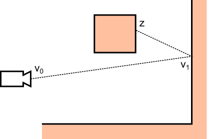
Let's take this vertex $\mathbf{z}$ and use it as vertex $\mathbf{z}_0$ to start an eye subpath. In order to use this virtual sensor with bidirectional path tracing, we need to define the following (see Veach eqn 10.7):

The area importance of the sensor $W_e(\mathbf{z}_0)$
The probability density wrt area $P_A(\mathbf{z}_0)$
The angular importance of the sensor $W_e(\mathbf{z}_0 \to \mathbf{z}_1)$
The probability density wrt projected solid angle $P_{\sigma^\perp}(\mathbf{z}_0 \to \mathbf{z}_1)$ .

The angular terms are defined by the BSDF at the surface. For our diffuse scene, each intersection point has a Lambertian BRDF with some reflectance $\rho$ , so our angular terms would be:

$$W_e(\mathbf{z}_0 \to \mathbf{z}_1) = \rho \\ P_{\sigma^\perp}(\mathbf{z}_0 \to \mathbf{z}_1) = \frac{1}{\pi}$$

The sensor has uniform area importance everywhere (i.e. $W_e(\mathbf{z}) = 1$ ), so the only part remaining is to compute the probability density wrt area $P_A(\mathbf{z})$ . As noted by Segovia et al, we compute this as a marginal probability density of all paths from the camera that can generate point $\mathbf{z}$ . For our diffuse scene with path $\overline{v} = \mathbf{v}_0 \mathbf{v}_1 \mathbf{z}$ , this is:

$$ P_A(\mathbf{z}) = \iint\limits_A \! P(\overline{v}) \, \mathrm{dA}(\mathbf{v}_1) \mathrm{dA}(\mathbf{v}_0) $$

Substituting the probability density of the path $\overline{v}$ and using the identity $\mathrm{d\sigma^\perp_{x^\prime}}(\widehat{\mathbf{x} - \mathbf{x^\prime}}) = G(\mathbf{x} \leftrightarrow \mathbf{x^\prime}) \mathrm{dA}(\mathbf{x})$ we get:

$$\begin{align*} P_A(\mathbf{z}) &= \iint\limits_A \! P(\overline{v}) \, \mathrm{dA}(\mathbf{v}_1) \mathrm{dA}(\mathbf{v}_0) \\ &= \iint\limits_A \! P_A(\mathbf{v}_0) P_A(\mathbf{v}_1|\mathbf{v}_0) P_A(\mathbf{z}|\mathbf{v}_1) \, \mathrm{dA}(\mathbf{v}_1) \mathrm{dA}(\mathbf{v}_0) \\ &= \iint\limits_A \! P_A(\mathbf{v}_0) P_{\sigma^\perp}(\mathbf{v}_0 \to \mathbf{v}_1) G(\mathbf{v}_0 \leftrightarrow \mathbf{v}_1) P_{\sigma^\perp}(\mathbf{v}_1 \to \mathbf{z}) G(\mathbf{v}_1 \leftrightarrow \mathbf{z}) \, \mathrm{dA}(\mathbf{v}_1) \mathrm{dA}(\mathbf{v}_0) \\ &= \int\limits_A \! \int\limits_\Omega \! P_A(\mathbf{v}_0) P_{\sigma^\perp}(\omega_0) P_{\sigma^\perp}(\mathbf{v}_1 \to \mathbf{z}) G(\mathbf{v}_1 \leftrightarrow \mathbf{z}) \, \mathrm{d\sigma^\perp}(\omega_0) \mathrm{dA}(\mathbf{v}_0) \end{align*}$$

Since we can't compute this integral analytically, we estimate it with importance sampling. Since $P_A(\mathbf{v}_0)$ and $P_{\sigma^\perp}(\omega_0)$ are probability densities themselves, sampling $\mathbf{v}_0$ and $\omega_0$ causes the function and pdf to cancel out, simplifying the estimate to:

$$ P_A(\mathbf{z}) \approx \frac{1}{N} \sum_{i=1}^N P_{\sigma^\perp}(\mathbf{v}_{i,1} \to \mathbf{z}) G(\mathbf{v}_{i,1} \leftrightarrow \mathbf{z}) \text{ for paths } \overline{v_i} = \mathbf{v}_{i,0} \mathbf{v}_{i,1} \mathbf{z} $$

Note this matches Segovia et al's equation 7, except we have derived this within the Veach framework so the notation is a bit different.

So in order to compute the probability density wrt area for any VPL location $\mathbf{z}$ , we construct N camera paths $\mathbf{v}_{i,0} \mathbf{v}_{i,1}$ , compute $P_{\sigma^\perp}(\mathbf{v}_{i,1} \to \mathbf{z})$ and $G(\mathbf{v}_{i,1} \leftrightarrow \mathbf{z})$ and use the equation above. Note that a path may estimate a zero pdf if either $P_{\sigma^\perp}$ or $G$ is zero. Considering our diffuse scene as before, here is an example for $N=4$ :

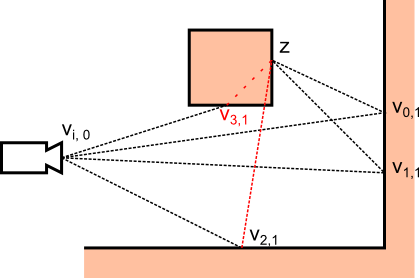
Multiple Camera Paths To Estimate PDF

In this example, only paths 0 and 1 would estimate a non-zero pdf. Path 2 returns 0 since $V(\mathbf{v}_{2,1} \leftrightarrow \mathbf{z}) = 0$ so $G(\mathbf{v}_{2,1} \leftrightarrow \mathbf{z}) = 0$ . Path 3 returns 0 since for a Lambertian BSDF $P_{\sigma^\perp}(\mathbf{v}_{3,i} \to \mathbf{z})$ is 0 for incoming and outgoing directions that are in opposite hemispheres.

If all paths produce a zero pdf estimate, we must conclude that the location is not possible to sample using camera paths. I don't think this is a problem, but we must take this into account during multiple importance sampling since it means the location is only reachable using light subpaths.

(Note: the sampling scheme for this virtual sensor is completely arbitrary, you could replace it or mix in any other sampling scheme and still use the same bidirectional construction of VPLs. For example, 10% of the time you could choose to sample from a surface in the scene using a precomputed CDF, and factor this into the pdf estimate. This would also ensure that VPL locations have a non-zero pdf estimate everywhere.)

Estimating $P_A(\mathbf{z})$ requires many intersection tests. To ensure good efficiency we should:

Reuse $\mathbf{v}_{i,0}$ and $\mathbf{v}_{i,1}$ for several VPLs (e.g. all VPLs generated in one pass)
Reuse all intersection tests used to compute $P_A(\mathbf{z})$ to also compute power brought to the camera for VPL resampling

Bidirectional Path Tracing

Now we have fully defined our virtual sensor we can use it with bidirectional path tracing. As usual we sample some light subpath $\mathbf{y}_0 \ldots \mathbf{y}_{S-1}$ and some eye subpath $\mathbf{z}_0 \ldots \mathbf{z}_{T-1}$ and consider all subpath combinations.

For each weighted contribution $C_{s,t}$ from a path formed from $s$ light subpath vertices and $t$ eye subpath vertices, we check $t$ to decide which VPL to accumulate the result into. If $t = 0$ , then this path is a light subpath that hit our virtual sensor, so use the VPL associated with vertex $\mathbf{y}_s$ . Otherwise, the path ends at the first eye subpath vertex so use the VPL associated with vertex $\mathbf{z}_0$ .

We also keep $y_0$ as a VPL for direct lighting, making the final total $S + 1$ VPLs. If we also handle the case where $\mathbf{z}_0$ happens to land on a light source (accumulating the emission into the VPL we already have at $\mathbf{z}_0$ ), we can multiple importance sample between these two cases (the ratio between pdfs is $P_A(\mathbf{y}_0)/P_A(\mathbf{z}_0)$ ).

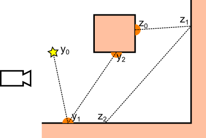
Here's an example for $S = T = 3$ , directly generating VPLs $\mathbf{y}_0$ , $\mathbf{y}_1$ , $\mathbf{y}_2$ and $\mathbf{z}_0$ by its subpath combinations. Note that the camera is only there to estimate $P_A(\mathbf{z})$ for some sampled or intersected point on our virtual sensor:

Example Bidirectional Path and Generated VPLs

Results?

As I mentioned in the introduction I'm going to resist posting any results until I can find some proper time for analysis, which will likely not be for a few weeks. This post exists so that someone can poke some holes in the theory, so I'd welcome any comments!