Bidirectional Path Tracing In Participating Media

15 Jul, 2012 #path-tracing #maths

The framework for integration over path space described by Veach REF1 can be extended to integrate over volumes (REF3 and REF4), using the original rendering equation as a boundary condition. An alternative framework was also developed by Lafortune in REF2. In the approaches described by these papers, scattering events are sampled according to the cumulative scattering density along a ray.

Here is some programmer art rendered using a brute force bidirectional path tracer that implements this approach, stopped at around 1000 samples per pixel.

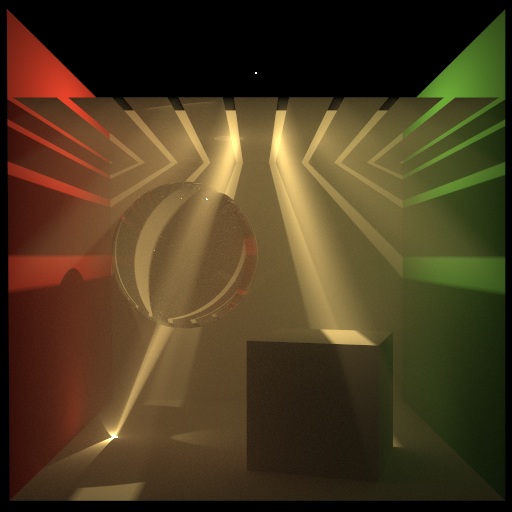
Cornell box with fog and volume caustics

Still noisy but working volume caustics, so achieves my goals. Since this is a brute force sampling (no MLT or manifolds) there are still issues with SDS paths that show up as unexpected bright spots on the glass sphere. If I manage to resurrect MLT code for REF5 I'll post an update.

This post is an attempt to gather together the definitions and equations for the weighted path contribution and MIS probability ratios for this sampling technique, as I've not seen this written down all in one place (with all of the interior terms of the weighted path contribution cancelled etc). Where possible I've tried to use similar notation to REF1, REF3 and REF4. This post is unapologetically maths-heavy!

$$ \newcommand{\x}{\mathbf{x}} \newcommand{\xp}{\mathbf{x^\prime}} \newcommand{\xpp}{\mathbf{x^{\prime\prime}}} \newcommand{\y}{\mathbf{y}} \newcommand{\z}{\mathbf{z}} \newcommand{\Vec}[1]{\overrightarrow{{#1}}} \newcommand{\sigp}{\sigma^\perp} \newcommand{\Pa}[1]{P_A({#1})} \newcommand{\Pv}[1]{P_V({#1})} \newcommand{\Psigp}[2]{{P_{\sigp}({#1} \to {#2})}} \newcommand{\Pbar}[2]{{\overline{P}({#1} \to {#2})}} \newcommand{\Pd}[2]{{P_d({#1} \to {#2})}} \newcommand{\Pns}[2]{{p_\text{noscat}({#1} \leftrightarrow {#2})}} \newcommand{\Pnrr}[2]{{p_\text{norr}({#1} \to {#2})}} \newcommand{\ds}{d_\text{scat}} \newcommand{\G}[2]{{G({#1} \leftrightarrow {#2})}} \newcommand{\V}[2]{{V({#1} \leftrightarrow {#2})}} \newcommand{\fs}[3]{{f_s({#1} \to {#2} \to {#3})}} \newcommand{\fp}[3]{{f_p({#1} \to {#2} \to {#3})}} \newcommand{\f}[3]{{f({#1} \to {#2} \to {#3})}} \newcommand{\Le}[2]{{L_e({#1} \to {#2})}} \newcommand{\We}[2]{{W_e({#1} \to {#2})}} \newcommand{\Trans}[2]{{\tau({#1} \leftrightarrow {#2})}} \newcommand{\d}[1]{{\mathop{\mathrm{d}{#1}}}} $$

Definitions

Notation	Meaning
$\y_0 \ldots \y_{s-1}$	Light subpath with $s$ vertices, starting at a light source.
$\z_0 \ldots \z_{t-1}$	Eye subpath with $t$ vertices, starting at a sensor.
$\overline{x}_{s,t}$	Full path from light source to sensor, vertices $\x_i$ formed from $s$ light subpath vertices and $t$ eye subpath vertices in the order $\y_0 \ldots \y_{s-1} \z_{t-1} \ldots \z_0$ .
$\Le{\x}{\xp}$	Emitted radiance from light source at $\x$ in direction of $\xp$ .
$\We{\x}{\xp}$	Emitted importance from sensor at $\x$ in direction of $\xp$ .
$\fs{\x}{\xp}{\xpp}$	BSDF at $\xp$ using the incoming and outgoing directions defined by $\x$ and $\xpp$ .
$N(\x)$	Normal direction at vertex $\x$ .
$\Vec{\x\xp}$	Unit direction from vertex $\x$ to vertex $\xp$ .
$\Pa{\x}$	Probability density wrt area of the vertex $\x$ (actually conditional probability assuming existence of the previous vertices of the subpath). Only used for vertices that are on surfaces.
$\Psigp{\x}{\xp}$	Probability density wrt projected solid angle of vertex $\xp$ from vertex $\x$ (again conditional on the previous vertices of the subpath).
$\Pnrr{\x}{\xp}$	Probability that the subpath is not terminated by Russian roulette between the vertices $\x$ and $\xp$ .
$\V{\x}{\xp}$	Visibility term between vertex $\x$ and vertex $\xp$ , 1 if unoccluded, 0 otherwise.
$\sigma_s(\x)$	Scattering density at position $\x$ .
$\sigma_a(\x)$	Absorption density at position $\x$ .
$\Pd{\x}{\xp}$	Probability density wrt distance of a scattering event at the vertex $\xp$ along the ray from vertex $\x$ .
$\Pns{\x}{\xp}$	Probability that no scattering event was sampled between the vertices $\x$ and $\xp$ .
$\fp{\x}{\xp}{\xpp}$	Scattering phase function at $\xp$ using the incoming and outgoing directions defined by $\x$ and $\xpp$ .
$\Pv{\x}$	Probability density wrt volume of the vertex $\x$ (again conditional on the previous vertices of the subpath). Only used for vertices that are particles in a volume.

Geometry Term

Following REF3 and REF4, first we need to slightly generalise the geometry term $\G{\x}{\xp}$ to allow for vertices that are particles:

$$ \G{\x}{\xp} = \V{\x}{\xp} \frac{D_\x(\Vec{\x\xp})D_\xp(\Vec{\xp\x})}{\|\x - \xp\|^2} $$

Where $D_\x(\omega)$ is defined by:

$$ D_\x(\omega) = \begin{cases} |N(\x) \cdot \omega|, & \text{if } \x \text{ is on a surface} \\ 1, & \text{if } \x \text{ is a particle} \end{cases} $$

Intuitively speaking, we consider the surface of a particle to always be exactly perpendicular to every ray that starts or ends there. This also allows us to treat solid angle (for example from sampling a phase function) as projected solid angle at particle vertices, since the projection is always trivial.

The geometry term is used in the following relationship between probability densities, assuming $\xp$ is a vertex on a surface:

$$ \Pa{\xp} = \Psigp{\x}{\xp} \, \G{\x}{\xp} $$

A similar identity can be used if $\xp$ is a particle in a volume:

$$ \Pv{\xp} = \Psigp{\x}{\xp} \, \G{\x}{\xp} \, \Pd{\x}{\xp} $$

Unlike (4) we don't include attenuation in the geometry term, since we want to have the geometry term cancel as usual between the measurement contribution function and its pdf.

Absorption, Scattering and Russian Roulette

We define $\Trans{\x}{\xp}$ to be the transmission along the ray between $\x$ and $\xp$ after energy is lost due to absorption and out-scattering:

$$ \Trans{\x}{\xp} = \exp \left( -\int_\x^\xp \! \left( \sigma_s(\z) + \sigma_a(\z) \right) \d{t} \right) $$

In the above integral, $t$ parameterises the ray between $\x$ and $\xp$ by distance, i.e. $\z = \x + t(\Vec{\x\xp})$ for $0 \le t \le \|\xp - \x\|$ .

When we extend a light or eye subpath, we use the following sampling technique:

Sample a ray direction using the BSDF, phase function or emission function at the current vertex (as usual for bidirectional path tracing). Russian roulette could also be applied to here to terminate the subpath.
Now we have a ray direction, sample $\sigma_s(\x)$ through just the medium along this ray, producing some distance $\ds$ and its pdf.
Cast the ray through the scene to find the first hit, using $\ds$ as the maximum ray distance to consider before giving up.
If we hit some geometry, we create a surface vertex at the intersection point as usual. If we did not hit any geometry, we create a volume vertex at distance $\ds$ along the ray.

When computing the contribution and weight of a particular path, we must be careful to include either the probability we did not scatter (for new surface vertices) or the probability density wrt distance of the scattering event (for new particle vertices), in addition to any other Russian roulette tests applied when sampling the ray direction. To apply all of this consistently, we will use a combined probability density $\overline{P}$ , defined as follows:

$$ \Pbar{\x}{\xp} = \Psigp{\x}{\xp} \, \Pnrr{\x}{\xp} \, \begin{cases} \Pns{\x}{\xp}, & \text{if } \xp \text{ is on a surface} \\ \Pd{\x}{\xp}, & \text{if } \xp \text{ is a particle} \end{cases} $$

Note that when $\x$ is also a particle, $\Psigp{\x}{\xp}$ is generated by sampling the phase function $f_p$ with respect to (non-projected) solid angle, which we can treat as projected solid angle since our particles are considered to always be perpendicular to rays connecting them.

Path Contribution

To implement bidirectional path tracing we first compute the unweighted contribution of the path, then compute its multiple importance sampling weight. The unweighted contribution is written as:

$$ C^\ast_{s,t} \equiv \frac{f_j(\overline{x}_{s,t})}{p_{s,t}(\overline{x}_{s,t})} $$

Vertices of a path can either be on a surface or a particle in a volume. As such, the measure for a path is now defined as:

$$ p_{s,t}(\overline{x}_{s,t}) = \prod_{i=0}^{s+t-1} \begin{cases} \Pa{\x_i}, & \text{if } \x_i \text{ is on a surface} \\ \Pv{\x_i}, & \text{if } \x_i \text{ is a particle} \end{cases} $$

As described by (1), we let the common terms of $f_j$ and $p_{s,t}$ cancel, allowing us to compute $C^\ast_{s,t}$ directly in the following form:

$$ C^\ast_{s,t} = \alpha^L_s \, c_{s,t} \, \alpha^E_t $$

If we update the $\alpha^L$ and $\alpha^E$ quantities to include particle vertices and transmission, they are defined by:

$$ \begin{align*} \alpha^L_0 & = 1 \\ \alpha^L_1 & = \frac{1}{\Pa{\y_0}} \\ \alpha^L_{i+1} & = \frac{\f{\y_{i-2}}{\y_{i-1}}{\y_i} \, \Trans{\y_{i-1}}{\y_i}}{\Pbar{\y_{i-1}}{\y_i}} \alpha^L_i \qquad \text{for } i \ge 1 \end{align*} $$

and

$$ \begin{align*} \alpha^E_0 & = 1 \\ \alpha^E_1 & = \frac{1}{\Pa{\z_0}} \\ \alpha^E_{i+1} & = \frac{\f{\z_{i-2}}{\z_{i-1}}{\z_i} \, \Trans{\z_{i-1}}{\z_i}}{\Pbar{\z_{i-1}}{\z_i}} \alpha^E_i \qquad \text{for } i \ge 1 \end{align*} $$

The function $f$ abstracts away whether vertices are particles or BSDF/emissive surfaces. For vertices at the start or end of a path it is defined as follows:

$$ \begin{align*} \f{\y_{-1}}{\y_0}{\y_1} & \equiv \Le{\y_0}{\y_1} \\ \f{\z_{-1}}{\z_0}{\z_1} & \equiv \We{\z_0}{\z_1} \end{align*} $$

and for interior vertices it is defined as:

$$ \f{\x}{\xp}{\xpp} = \begin{cases} \fs{\x}{\xp}{\xpp}, & \text{if } \xp \text{ is on a surface} \\ \sigma_s(\xp) \, \fp{\x}{\xp}{\xpp}, & \text{if } \xp \text{ is a particle} \end{cases} $$

The final term $c_{s,t}$ in the path contribution is defined by:

$$ \begin{align*} c_{0,t} & = \Le{\z_{t-1}}{\z_{t-2}} \\ c_{s,0} & = \We{\y_{s-1}}{\y_{s-2}} \\ c_{s,t} & = \f{\y_{s-2}}{\y_{s-1}}{\z_{t-1}} \, \G{\y_{s-1}}{\z_{t-1}} \, \Trans{\y_{s-1}}{\z_{t-1}} \, \f{\y_{s-1}}{\z_{t-1}}{\z_{t-2}} \end{align*} $$

where the last definition is only used when $s > 0$ and $t > 0$ .

Multiple Importance Sampling

The path contribution $C^\ast_{s,t}$ is weighted by the multiple importance sample weight $w_{s,t}$ before being accumulated into the output image. Veach describes how this can be achieved just by looking at the probability ratios.

If we consider the full path $\overline{x}_{s,t} = \x_0 \ldots \x_k$ for $k=s+t-1$ , then there are $k+2$ possible combinations of subpaths that could construct this path, corresponding to $0 \le s \le k+1$ . If we label the probability of each combination as $p_i$ , we can define the weight $w_{s,t}$ in terms of the ratios between these $p_i$ .

For example, for the power heuristic with power $\beta$ , the weight is computed as:

$$ w_{s,t} = \frac{p^\beta_s}{\sum^{k+1}_{i=0} p^\beta_i} = \frac{1}{\sum^{k+1}_{i=0} (p_i/p_s)^\beta} $$

If we extend the Veach definition of these ratios from (1) to include vertices that are particles in a volume, we get the following:

$$ \begin{align*} \frac{p_1}{p_0} & = \frac{\Pa{\x_0}}{\Pbar{\x_1}{\x_0} \, \G{\x_1}{\x_0}} \\ \frac{p_{i+1}}{p_i} & = \frac{\Pbar{\x_{i-1}}{\x_i} \, \G{\x_{i-1}}{\x_i}}{\Pbar{\x_{i+1}}{\x_i} \, \G{\x_{i+1}}{\x_i}} \qquad \text{for } 0 < i < k \\ \frac{p_{k+1}}{p_k} & = \frac{\Pbar{\x_{k-1}}{\x_k} \, \G{\x_{k-1}}{\x_k}}{\Pa{\x_k}} \end{align*} $$

References

Robust Monte Carlo Methods for Light Transport Simulation by Eric Veach.
Rendering Participating Media with Bidirectional Path Tracing by Eric Lafortune and Yves Willems.
Metropolis Light Transport for Participating Media by Mark Pauly, Thomas Kollig and Alexander Keller.
Manifold Exploration: A Markov Chain Monte Carlo technique for rendering scenes with difficult specular transport by Wenzel Jakob and Steve Marschner.
Simple and Robust Mutation Strategy for Metropolis Light Transport Algorithm by Csaba Kelemen and László Szirmay-Kalos.